MAG generation
Generation of metagenome assembled genomes (MAGs) from assemblies
Assessment of quality (MIGMAGs)
Taxonomic assignment
Comparison to public genomes
Prerequisites
For this tutorial you will need to first setup the docker container by running:
cd /course/metagenomics-data/mag_generation/data
docker run --rm -it -v $(pwd):/opt/data quay.io/microbiome-informatics/holofood-course-2022-mag-generation:latest
cd /opt/data
mkdir obs_results
 You will notice the outputs of assembly, binning and checkM have been pre-generated for you.
Since some of these processes can take ~1hr we have provided the results to save time. To view the available data run:
You will notice the outputs of assembly, binning and checkM have been pre-generated for you.
Since some of these processes can take ~1hr we have provided the results to save time. To view the available data run:
ls /opt/data
Assembling data
Learning Objectives - in the following exercises an assembled HoloFood salmon gut sample has been provided.
You will assess the quality of these assemblies, which are used later to generate bins.
Once quality control of sequence reads is complete, you may want to perform de novo assembly in addition to, or as an alternative to a read-based analyses. The first step is to assemble your sequences into contigs. There are many tools available for this, such as MetaVelvet, metaSPAdes, IDBA-UD, MEGAHIT. We generally use metaSPAdes, as in most cases it yields the best contig size statistics (i.e. more continguous assembly) and has been shown to be able to capture high degrees of community diversity (Vollmers, et al. PLOS One 2017). However, you should consider the pros and cons of different assemblers, which not only includes the accuracy of the assembly, but also their computational overhead. For example, very diverse samples with a lot of sequence data uses a lot of memory with metaSPAdes.
The assembly step has been run for you. To run metaSPAdes we executed the following commands (but don’t run it now!):
mkdir assemblies
metaspades.py -t 4 --only-assembler -m 10 -1 reads/ERR4918566_1.fastq.gz -2 reads/ERR4918566_2.fastq.gz -o assemblies
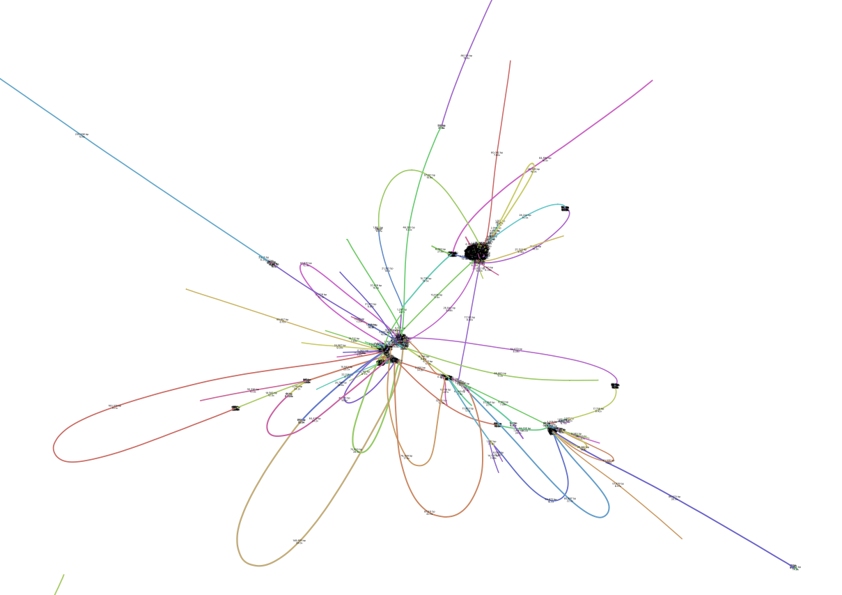
MetaSPAdes also produces assembly graphs which can be visualised using tools such as Bandage. Parts of the assembly graph from the above assembly are shown below.
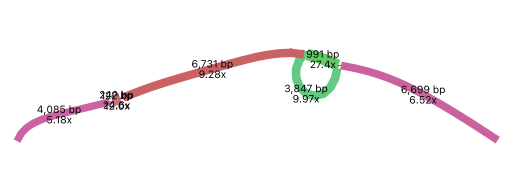
The simplest graph would contain a single long contig but this is not always the case.
The graph on the left is made up of several kmers. It also contains a “bubble” which could be repeated sequences appearing as single nodes with multiple inputs and outputs.
The right hand graph is very complex and difficult to resolve.
Assessing genome quality
Assemblies can contain contamination from several sources e.g. host, human, PhiX and so on.
PhiX, is a small bacteriophage genome typically used as a calibration control in sequencing runs. Most library preparations will use PhiX at low concentrations, however it can still appear in the sequencing run. If not filtered out, PhiX can form small spurious contigs which could be incorrectly classified as diversity.
 Lets assess the resulting assembly contigs file. Run the following to make a PhiX reference database,
followed by blast to identify PhiX contigs in our assembly file:
Lets assess the resulting assembly contigs file. Run the following to make a PhiX reference database,
followed by blast to identify PhiX contigs in our assembly file:
# make reference database
makeblastdb -in assemblies/decontamination/phiX.fna -input_type fasta -dbtype nucl -parse_seqids -out obs_results/phix_blastDB

# run blast
blastn -query assemblies/ERR4918566.fasta -db obs_results/phix_blastDB -task megablast -word_size 28 -best_hit_overhang 0.1 -best_hit_score_edge 0.1 -dust yes -evalue 0.0001 -min_raw_gapped_score 100 -penalty -5 -soft_masking true -window_size 100 -outfmt 6 -out obs_results/ERR4918566.blast.out
View the blast results
cat obs_results/ERR4918566.blast.out
Use the following link to understand what is in each column https://www.metagenomics.wiki/tools/blast/blastn-output-format-6
 Are there any significant hits?
What are the lengths of the matching contigs?
We would typically filter metagenomic contigs at a length of 500bp. Would any PhiX contamination remain after this filter?
Within the /opt/data/assemblies folder there is a second cleaned contigs file with contigs <500bp filtered out and contamination removed.
Lets assess the statistics of assemblies before and after quality control.
gunzip assemblies/ERR4918566_clean.fasta.gz

# statistics before quality control
assembly_stats assemblies/ERR4918566.fasta > obs_results/assembly_stats.json

# statistics after quality control
assembly_stats assemblies/ERR4918566_clean.fasta > obs_results/assembly_stats_clean.json
This will output two simple tables in JSON format, but it is
fairly simple to read. To view each file you can open it via the folders or run:
cat obs_results/assembly_stats.json
cat obs_results/assembly_stats_clean.json
Looking at the ‘Contig stats’ for both, what is the length of longest and shortest contigs before and after
quality control?
What is the N50 of the two assembly files? Given that the input
sequences were ~150bp long paired-end sequences, what does this tell you
about the assembly?
N50 is a measure to describe the quality of assembled genomes
that are fragmented in contigs of different length. We can apply this
with some caution to metagenomes, where we can use it to crudely assess
the contig length that covers 50% of the total assembly. Essentially
the longer the better, but this only makes sense when thinking about
alike metagenomes. Note, N10 is the minimum contig length to cover 10
percent of the metagenome. N90 is the minimum contig length to cover 90
percent of the metagenome.
Now take the first 40 lines of the first sequence and perform a blast search.
To select the first 40 lines perform the following:
# the number selected is 41 to allow for the header
head -n 41 assemblies/ERR4918566_clean.fasta > obs_results/subset_contigs.fasta
Load NCBI in the browser https://blast.ncbi.nlm.nih.gov/Blast.cgi and choose Nucleotide:Nucleotide. Upload the subset sequence file. Click ‘Choose file’.
Navigate to the file: ‘Other locations’ –> ‘Computer’ –> ‘course’ –> ‘metagenomics-data’ –> ‘mag_generation’ –> ‘obs_results’ –> ‘subset_contigs.fasta’
Leave all other options as default on the search page.
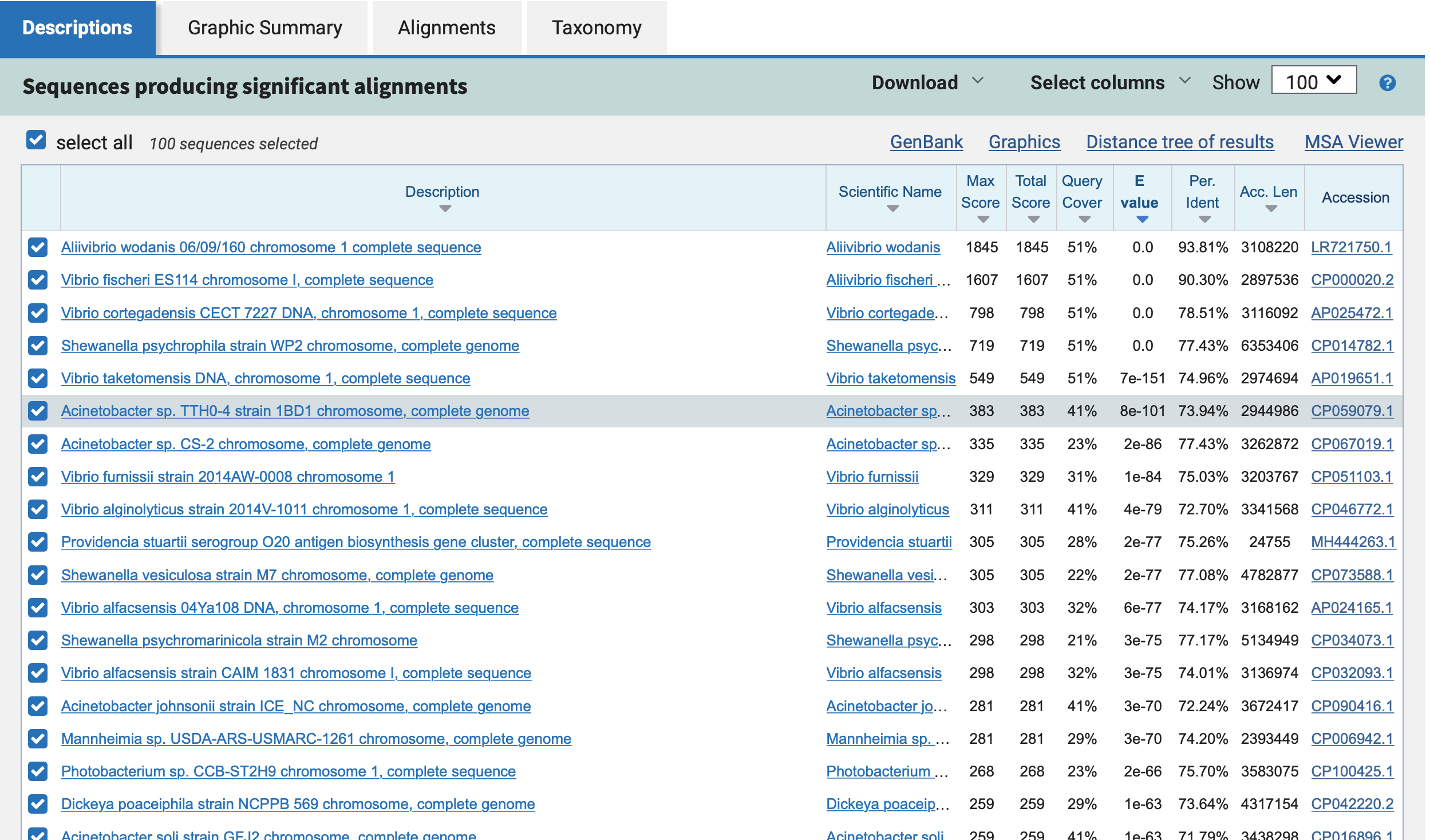
Which species do you think this sequence may be coming from?
Generating metagenome assembled genomes (MAGs)
Learning Objectives - in the following exercises you will:
look at some outputs binning
assess the quality of the genomes using checkM
remove redundancy among genomes
visualise a placement of these genomes within a reference tree.
Binning
As with the assembly process, there are many software tools available for
binning metagenomic assemblies. Examples include, but are not limited to:
MaxBin: https://sourceforge.net/projects/maxbin
CONCOCT: https://github.com/BinPro/CONCOCT
MetaBAT: https://bitbucket.org/berkeleylab/metabat
MetaWRAP: https://github.com/bxlab/metaWRAP
There is no clear winner between these tools, so the best approach is to experiment and compare a few different ones to determine which works best for your dataset.
For this exercise the bins have been generated using metaWRAP which uses a combination of the 3 tools above. However we have also provided the output of MetaBAT for the assembly above. The way in which MetaBAT bins contigs together is summarised in the figure below.
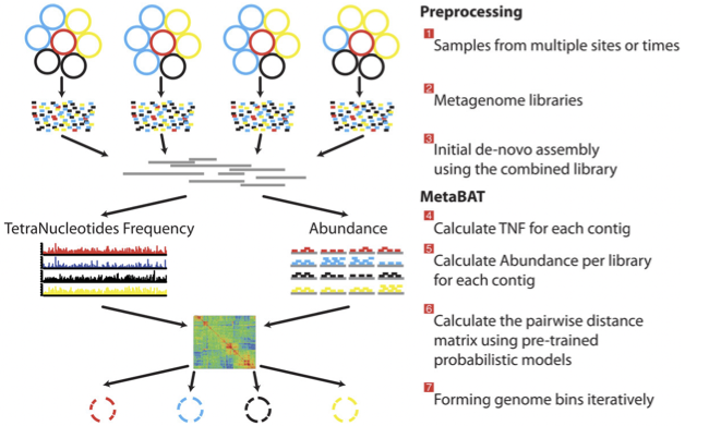
MetaBAT workflow (Kang, et al. PeerJ 2015).
The binning step has been run for you. To run MetaBAT we executed the following commands (but don’t run it now!):
Prior to running , we generated coverage statistics by mapping reads to the contigs. To do this, we used bwa (http://bio-bwa.sourceforge.net/) and then the samtools software (http://www.htslib.org) to reformat the output.
# index the contigs file that was produced by metaSPAdes:
bwa index ERR4918566_clean.fasta

# map the original reads to the contigs:
bwa mem ERR4918566_clean.fasta ERR4918566_1.fastq.gz ERR4918566_2.fastq.gz > input.fastq.sam

# reformat the file with samtools:
samtools view -Sbu input.fastq.sam > junk
samtools sort junk input.fastq.sam

# calculate coverage depth for each contig
jgi_summarize_bam_contig_depths --outputDepth contigs.fasta.depth.txt input.fastq.sam.bam

# run MetaBAT
metabat2 --inFile ERR4918566_clean.fasta --outFile ERR4918566_metabat/bin --abdFile contigs.fasta.depth.txt
Once the binning process is complete, each bin will be grouped into a multi-fasta file with a name structure of
bin.[0-9].fa.
Inspect the output of the binning process.
ls bins/ERR4918566_metabat/metabat2_bins

# count sequences in each bin
grep -c '>' bins/ERR4918566_metabat/metabat2_bins/*.fa
How many bins did the process produce?
How many sequences are in each bin?
We have provided you with a subset of bins from several HoloFood salmon sample assemblies, including one co-assembly.
ls bins/*.fa
Assessing genome quality
Not all bins will have the same level of accuracy since some
might represent a very small fraction of a potential species present in
your dataset. To further assess the quality of the bins we will use
CheckM.
CheckM has its own reference database of single-copy marker genes. Based on the proportion of these markers detected in the bin, the number of copies of each and how different they are, it will determine the level of completeness, contamination and strain heterogeneity of the predicted genome. Once again, this can take some time, so we have run it in advance. To repeat the process, you would run the following command:
# This program has some handy tools not only for quality control, but also for taxonomic classification, assessing coverage, building a phylogenetic tree, etc. The most relevant ones are wrapped into the lineage_wf workflow.
checkm lineage_wf -x fa bins/ checkM/checkm_output/ --tab_table -f checkM/bins_qa.tab -t 4
To inspect the summary output file of checkM:
cat checkM/bins_qa.tab
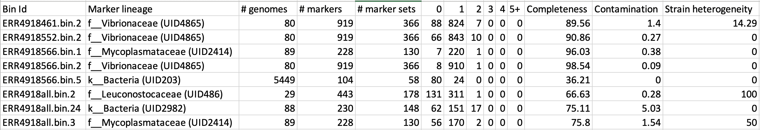
Example output of CheckM
This file contains the taxonomic assignment and quality assessment of each
bin with the corresponding level of
completeness, contamination and strain heterogeneity A quick way to infer the overall quality of the bin is to calculate the quality score:
(completeness - 5*contamination).
You should be aiming for an minimum score of at
least 50%. Whereby if the genome is only 50% complete, contamination must be 0.
Based on the above formula for quality score, how many genomes pass this filter?
Do any of the genomes have a similar taxonomic annotation? What might this mean?
Getting species representatives
Next we will de-replicate our genomes to generate species level clusters and select a representative MAG per species.
We will use dRep to do this. dRep can rapidly and accurately compare a list of genomes in a pair-wise manner.
This allows identification of groups of organisms that share similar DNA content in terms of Average Nucleotide Identity (ANI).
To prepare for de-replication:
# identify bins with a minimum quality score of 50 and generate csv summary
echo "genome,completeness,contamination" > obs_results/quality.csv
awk -F "\t" -v OFS=',' '{ if ($12 - ($13 * 5) >= 50) print $1".fa",$12,$13}' checkM/bins_qa.tab >> obs_results/quality.csv

# copy bin folder to our output folder
cp -r bins/ obs_results/
# filter lower quality bins into a separate folder
mkdir obs_results/poor-bins
mv obs_results/bins/ERR4918566.bin.5.fa obs_results/poor-bins/
mv obs_results/bins/ERR4918all.bin.24.fa obs_results/poor-bins/
Now run dRep with this command:
dRep dereplicate obs_results/drep/ -g obs_results/bins/*.fa -pa 0.9 -sa 0.95 -nc 0.6 -cm larger --genomeInfo obs_results/quality.csv -comp 50 -con 5
Using the following manual https://drep.readthedocs.io/en/latest/module_descriptions.html#dereplicate can you identify the ANI and coverage thresholds used to compare the genomes?
Inspect the output files:
# The folder of representative genomes per species
ls obs_results/drep/dereplicated_genomes/

# The cluster and score of de-replicated genomes
cat obs_results/drep/data_tables/Wdb.csv

# Pair-wise Mash comparison results of all bins
cat obs_results/drep/data_tables/Mdb.csv
How many species representative MAGs were produced?
Taxonomic Classification
Finally we will look at the taxonomic assignments of our species representative MAGs
This can be done in a few different ways. One example is the checkM lineage_wf analysis perfomed above which also produces a reference tree which can be found in checkM/checkm_output/storage/tree/concatenated.tre.
However we will compare our genomes to the genome taxonomy database (GTDB). GTDB is a standardised microbial taxonomy based on genome phylogeny. GTDB phylogeny is constructed using a mixture of isolate genomes and MAGs obtained from RefSeq and GenBank. The GTDB-Tk toolkit performs a rapid classification producing a multiple sequence alignment to the GTDB reference genomes and best lineage matches.
For the purpose of this practical, we have used the 3 salmon gut MAGs generated today and a set of other HoloFood chicken ileum and salmon MAGs to generate a phylogenetic tree. We have run GTDB-Tk in advance with all the mentioned genomes. To repeat the process, you would run the following commands (don’t run this now!):
# running the gtdb workflow
gtdbtk classify_wf --cpus 2 --genome_dir folder-of-genomes/ --out_dir tree/ -x fa

# generate a phylogenetic tree using the multiple sequence alignment
iqtree2 -nt 16 -s tree/gtdbtk.bac120.user_msa.fasta
Inspect the GTDB files:
# first exit the docker container
exit

# navigate to the output directory
cd /course/metagenomics-data/tree
The GTDB-tk summary file /course/metagenomics-data/tree/gtdbtk.bac120.summary.tsv contains all the genomes from chicken ileum and salmon.
View the GTDB output for the salmon MAGs generated today:
# select the 3 MAGs
head -n1 gtdbtk.bac120.summary.tsv > mags_taxonomy.tsv
grep -E 'ERR4918566_bin.1|ERR4918566_bin.2|ERR4918all_bin.2' gtdbtk.bac120.summary.tsv >> mags_taxonomy.tsv
cat mags_taxonomy.tsv
Are any MAGs classified to the species level? For this MAG what is the closest reference genome in GTDB.
Search the reference genome in https://gtdb.ecogenomic.org Is it derived from an isolate or MAG?
Visualising the phylogenetic tree
We will now plot and visualize the tree we have produced. A quick and user- friendly way to do this is to use the web-based interactive Tree of Life (iTOL): http://itol.embl.de/index.shtml
To use iTOL you will need a user account, or we have already created a tree you can visualise.
The login is as follows:
User: EBI_training
Password: EBI_training
After you login, just click on My Trees in the toolbar at the top and select
holofood.bac120.treefile from the Imported trees workspace.
Alternatively, if you want to create your own account and plot the tree yourself follow these steps:
1) After you have created and logged in to your account go to My Trees
- 2) From there select Upload tree files and locate the tree to upload in the path:
Navigate to the file: ‘Other locations’ –> ‘Computer’ –> ‘course’ –> ‘metagenomics-data’ –> ‘tree’ –> ‘gtdbtk.bac120.user_msa.fasta.treefile’
3) Once uploaded, click the tree name to visualize the plot.
You will find several annotation files starting “itol” in the same folder as above
4) To colour the clades and the outside circle according to the phylum of each genome, drag and drop the files itol_gtdb-legend.txt onto the tree.
5) To colour outer ring according to “novelty” drag and drop the file itol_gtype-layer.txt onto the tree. “Novel” is shown in green and refers to genomes not classified to species level in GTDB. “Existing” is in blue.
6) Reformat the tree to see the labels: On the basic control panel select Labels - Display and Label options - At tips
7) Finally to highlight the 3 MAGs produced today, drag and drop the files itol_mags-bold.txt onto the tree.
Feel free to play around with the plot.
What is the genome most closely related to our salmon MAG ERR4918566 bin.2?
Can you find the taxonomic lineage for this genome in the GTDB output file /course/metagenomics-data/tree/gtdbtk.bac120.summary.tsv?
Hint
Replace the space with ‘_’ when searching the file.
Compare genomes to public MAG catalogue in MGnify
We can compare our newly generated MAGs to existing public MAG catalogues on MGnify.
Open a new Terminal on your virtual desktop (you’re no longer using the Docker container).
Load the Jupyter Notebook that we’ve prepared for you:
hf-conda-setup
conda activate jupyter
cd /course/docs/sessions/metagenomics/notebooks/
jupyter lab
This should open a Jupyter Lab in the browser (Firefox). If Firefox doesn’t open by itself, click one of the links printed in the Terminal, or copy-paste one into Firefox.
Find the Compare MAGs to MGnify.ipynb notebook in the left hand panel, and open it. Follow the instructions in the Notebook.
Do any of your MAGs match a known species in the human gut catalogue on MGnify?